Quick start
This walks through a complete analysis of a mixture of two species, malic acid
(residue name MAL) and 2-methylerythritol (MOL), simulated with GROMACS.
1. What you need
- A topology with residue names, masses, partial charges and bonds: a GROMACS
.tpr, a CHARMM/NAMD.psfor a LAMMPS DATA file (atom_style full) has them all; a.groor.pdbdoesn't. The residues must be numbered 1 to N in topology order (see Troubleshooting). - A trajectory MDAnalysis can read (
.xtc,.trr,.dcd, a LAMMPS dump, ...), with the box, so distances respect periodic boundary conditions. - A configuration file saying which molecules connect to which.
2. Write the configuration
Save this as config.yml:
rules:            # which residue pairs connect, and how
  MAL:
    MAL: hb d 3.5 a 120   # hydrogen bond: donor-acceptor <= 3.5 Å, D-H-A angle >= 120°
    MOL: cm 6.0           # centers of mass closer than 6 Å
  MOL:
    MOL: cm 6.0

solute: [MAL]      # the species of interest
nucleus: [solute]  # nuclei: connected groups of solutes inside each cluster
follow: [solute]   # one coordinate file per solute molecule
solvent isn't given, so every residue name in rules that isn't a solute (here
MOL) is the solvent. Every key is described in Configuration.
3. Run it
The terminal shows what was understood before the run starts, a progress bar, and a summary at the end:
12:57:55 | INFO     | System: 3600 atoms in 200 residues (100 MOL, 100 MAL)
12:57:55 | INFO     | Trajectory: 53 frame(s) from 0 to 49920 ps, every 960 ps
12:57:55 | INFO     | Box (first frame): 324.60 x 324.60 x 324.60 angstrom
12:57:55 | INFO     | Topology has no elements, guessing them from atom names
12:57:55 | INFO     | Effective configuration:
rules (distances in angstrom, angles in degrees):
  MAL - MAL: hb d 3.5 a 120.0 hmin 0.9 hmax 1.1 hq 0.3 aq -0.5
  MAL - MOL: cm 6.0
  MOL - MOL: cm 6.0
solute: MAL
solvent: MOL
nucleus: MAL
follow: solute (one solute-<resid>.gro per solute)
...
analyses: SizeEvolution, Lineage, SoluteSolvent, ClusterCoordinates, Nucleus, JsonReport
report_compression: zstd (molclusters.jsonl.zst)
12:57:55 | INFO     | Tracking clusters over 53 frame(s)
100%|##########| 53/53 [00:07<00:00,  7.03it/s]
12:58:02 | INFO     | Connections per frame, by rule: MAL - MAL (hb ...) 42.2, MAL - MOL (cm 6.0) 37.5, MOL - MOL (cm 6.0) 12.8
12:58:02 | INFO     | [SizeEvolution] Found 23.3 cluster(s) per frame on average (0-32); the largest held 81 molecule(s).
12:58:02 | INFO     | [Lineage] Cluster lineage: 120 cluster(s) formed of free molecules and 719 split off others; ...
12:58:03 | INFO     | Results written to results: evo.txt, cluster_events.csv, cluster_lifetimes.csv, ...
Check the effective configuration
The Effective configuration block shows the rules with their defaults filled
in, the solute keyword expanded and the analyses that will run. It is the
quickest way to catch a misspelled residue name or a cutoff in the wrong unit.
The Connections per frame, by rule line at the end tells you whether each
rule actually connected anything.
4. Look at the results
The results folder now holds:
| File | Contents |
|---|---|
evo.txt |
number of clusters and their minimum, average and maximum size, per frame |
cluster_events.csv |
every formation, split, merge and dissolution |
cluster_lifetimes.csv |
each cluster's birth, end, lifetime, origin and fate |
solute_solvent.csv |
the clusters holding both solutes and solvents, averaged per frame |
nucleus_data.csv |
the nuclei inside the clusters, averaged per frame |
coordinates/*.gro |
the clusters holding solutes, made whole, as GROMACS coordinate files |
molclusters.jsonl.zst |
every cluster of every frame, with its properties and connections |
molclusters_<date>_<time>.log |
the log of the run (and a .json copy) |
For instance, plotting the number of clusters and the size of the largest one over
time, from evo.txt (with matplotlib, installed
separately):
import numpy as np
import matplotlib.pyplot as plt

time, n_clusters, min_size, avg_size, max_size = np.loadtxt("results/evo.txt", unpack=True)

fig, (top, bottom) = plt.subplots(2, 1, sharex=True)
top.plot(time / 1000, n_clusters)
top.set_title("Number of clusters", loc="left")
bottom.plot(time / 1000, max_size, color="C1")
bottom.set_title("Largest cluster (molecules)", loc="left")
bottom.set_xlabel("Time (ns)")
plt.show()
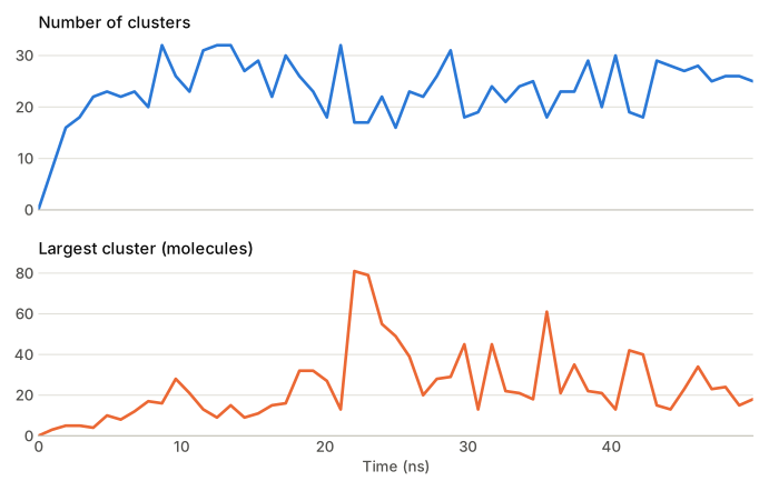
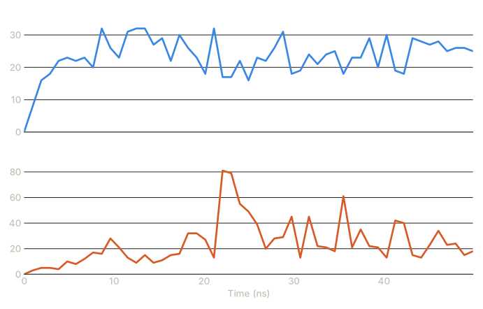
The two quantities are counts of different things (clusters, and molecules in one cluster), so each gets its own panel rather than sharing an axis.
Every cluster of every frame is in the report, which reads as one table:
from molclusters.report import read_report

clusters = read_report("results/molclusters.jsonl.zst").clusters()
print(clusters[["time", "id", "size", "radius", "density", "dipole_moment"]])
         time   id  size    radius   density  dipole_moment
0       960.0    1     3  6.005953  0.736076       6.543105
1       960.0    2     2  4.611475  1.084071       7.514518
2       960.0    3     2  4.888258  0.910154       4.044914
3       960.0    4     2  5.473106  0.648448       7.408297
4       960.0    5     2  5.301664  0.713412       2.192518
...       ...  ...   ...       ...       ...            ...
1229  49920.0  835     2  5.200793  0.761538       8.052136
1230  49920.0  836     2  5.154270  0.782346       6.681270
1231  49920.0  837     2  5.029856  0.841848       6.834615
1232  49920.0  838     2  5.216615  0.760383       0.000000
1233  49920.0  839     2  5.298673  0.725600       0.000000

[1234 rows x 6 columns]
Where to go next:
- How clusters are tracked, to know what the ids and events mean;
- Output files and The JSON report, column by column;
- Configuration, for the other rule options and keys.